Year_of_Release <- c("1997","1999","2001","2002","2003","2004","2006","2007","2007","2008")

Film <- c("Titanic",
          "Star Wars:Episode I-The Phantom Menace",
          "Harry Potter and the Sorcerer's Stone",
          "The Lord of Rings:The Two Towers",
          "The Lord of Rings:The Return of the King",
          "Shrek 2",
          "Pirates of the Carribean:Dead Man's Chest",
          "Pirates of the Carribean:At World's End",
          "Harry Potter and the Order of the Phoenix",
          "The Dark Knight")

Production_Budget <- c(1.84,0.92,0.98,0.93,1.12,0.92,1.07,0.96,0.94,0.95)Code & Implementation
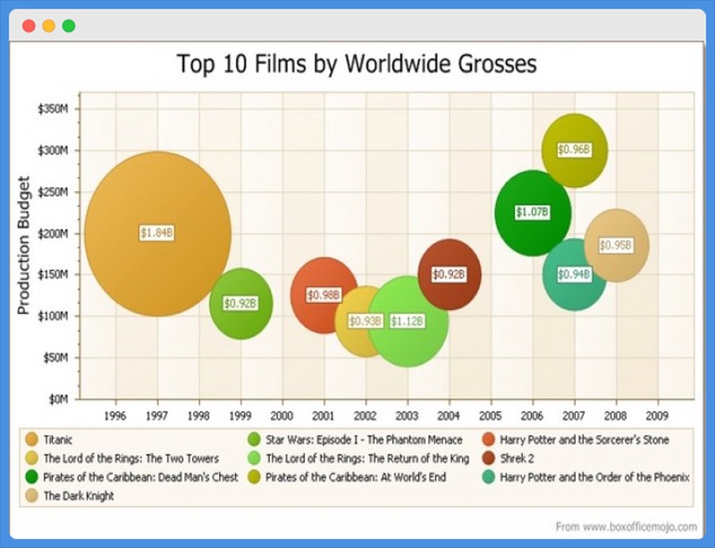
Data analysed from the graph
filmdata <- data.frame(Year_of_Release,Film,
                       Production_Budget)
filmdata
Year_of_Release Film Production_Budget
1 1997 Titanic 1.84
2 1999 Star Wars:Episode I-The Phantom Menace 0.92
3 2001 Harry Potter and the Sorcerer's Stone 0.98
4 2002 The Lord of Rings:The Two Towers 0.93
5 2003 The Lord of Rings:The Return of the King 1.12
6 2004 Shrek 2 0.92
7 2006 Pirates of the Carribean:Dead Man's Chest 1.07
8 2007 Pirates of the Carribean:At World's End 0.96
9 2007 Harry Potter and the Order of the Phoenix 0.94
10 2008 The Dark Knight 0.95Libraries
library(ggplot2)
library(plotly)
Redesign 1
Plot3 = ggplot(filmdata, aes( x=Year_of_Release,y=Production_Budget))+
  geom_bar(stat = "identity", color="black",aes(fill = Film),position = "dodge")+
  scale_y_continuous(limits=c(0,2))+
  labs(x ="Release Year",y="Production Budget in Billions",title ="Top 10 Films by Worldwide Grosses")+
  scale_fill_manual(values = c(rgb(0,0.3,0),"grey","yellow","skyblue","orange","blue","purple","green","pink","red"))+
  theme(legend.text=element_text(size=8,face="italic"),
        legend.title=element_text(size=8.5,face="bold"),
        plot.title=element_text(size=10,face="bold",hjust=0.5),
        axis.title=element_text(size=8.5,face="bold"))

Plot3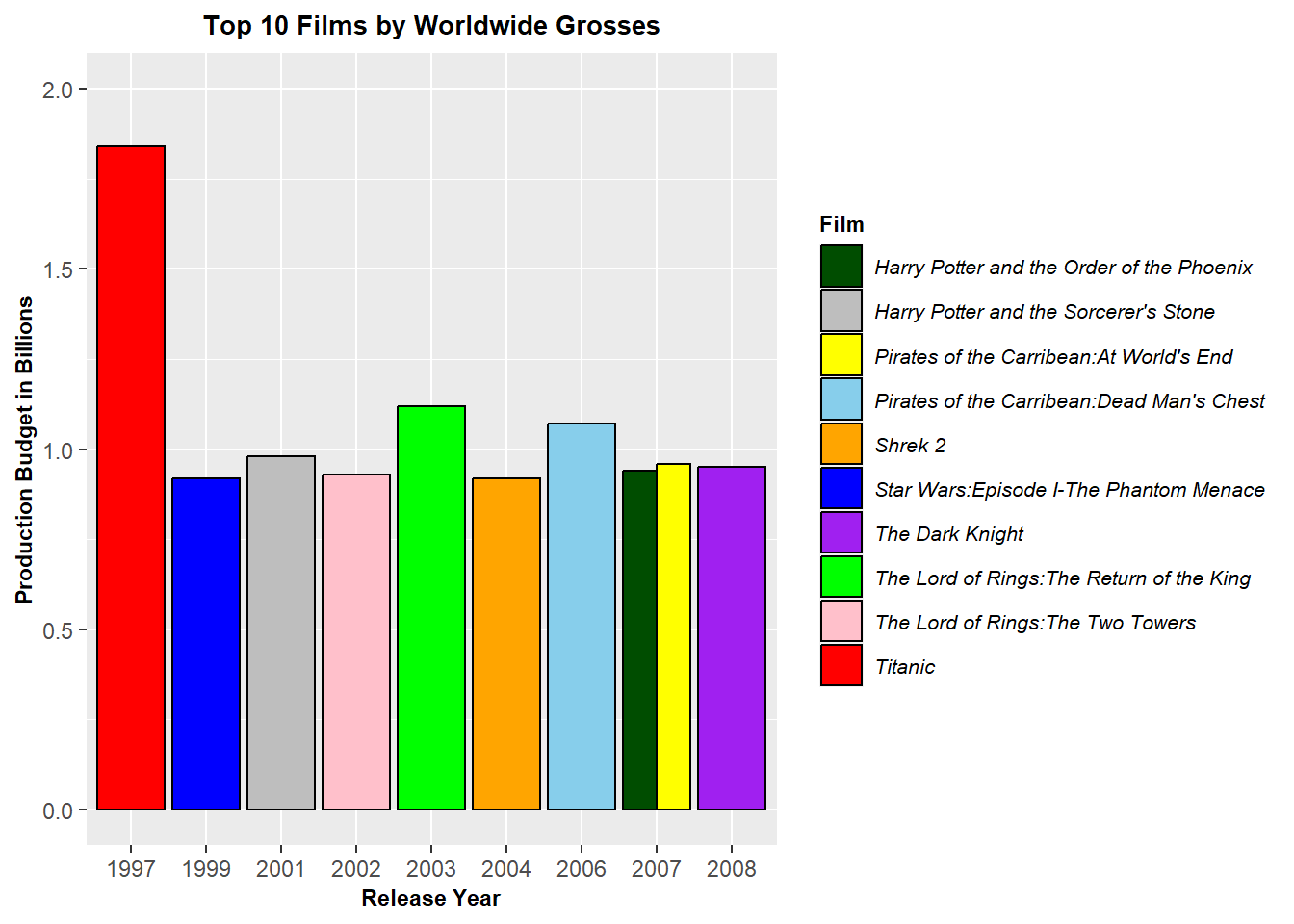
Using ggplotly to make the above graph interactive.
ggplotly(Plot3)Redesign 2
Plot4 = ggplot(filmdata, aes(x = Year_of_Release, y = Production_Budget)) +
  geom_point(aes(color = Film))+
  scale_y_continuous(limits = c(0,2), breaks = seq(0,2,.1))+
  labs(x ="Release Year",y="Production Budget in Billions",title ="Top 10 Films by Worldwide Grosses")+
  scale_color_manual(values = c(rgb(0,0.5,0),"maroon","yellow","skyblue","orange","blue","purple","green","pink","red"))+
  theme(legend.text=element_text(size=8,face="italic"),
        legend.title=element_text(size=8.5,face="bold"),
        plot.title=element_text(size=10,face="bold",hjust=0.5),
        axis.title=element_text(size=8.5,face="bold"))

Plot4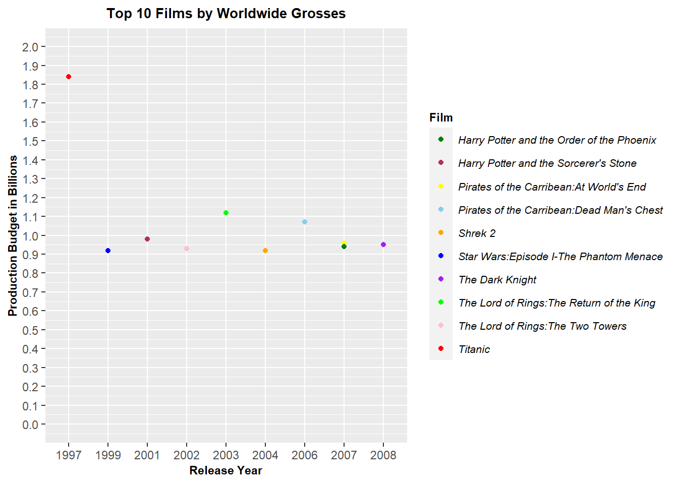
Using ggplotly to make the above graph interactive.
ggplotly(Plot4)